Our Data = Your Data. Explore. Have Fun.
Each figure below is interactive
Rotate/pan by clicking and dragging
Zoom in/out by scrolling with the mouse (using two fingers with the touch pad)
Our 1st research goal:
Use genetic data to determine which routes
the small cabbage white butterfly took
as it spread across the world over the last ~160 years.
Think of it as 23&Me but with butterflies.
Step 1. Obtain butterflies from all over the world.
With the help of hundreds of participants we were able to get thousands of butterflies from all over the world. We then extracted DNA from a subset of those butterflies. Using that DNA we sequenced parts of each butterfly's nuclear and mitochondrial genome. Like humans, each butterfly has a nuclear and mitochondrial genome and they provide information about the ancestry of that butterfly (find out more here).
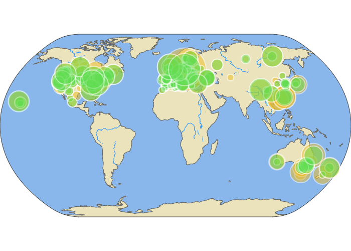
Here you can see our sample sizes--the number of butterflies that had portions of their nuclear and mitochondrial genomes sequenced.
Scroll over the map to see how many individuals were sequenced from each location. You can also click and drag the map to move around the world.
Step 2. Determine how many genetically distinct populations exist in the world.
We did this using the (nuclear) genetic data we extracted from each butterfly. Why do we need to do this? The simple answer is that the evolutionary models we use to understand genetic patterns are designed with populations in mind. It is also the case that our resolution for determining the source of a population will depend on whether we can tell them apart genetically. That is, if we have a butterfly from North America and want to know if it came from Europe or Asia, the butterflies in Europe and Asia have to be genetically distinct from each other. Think of it as butterfly forensics. If the DNA of every suspect look the same we won't be able to know which is the real culprit.
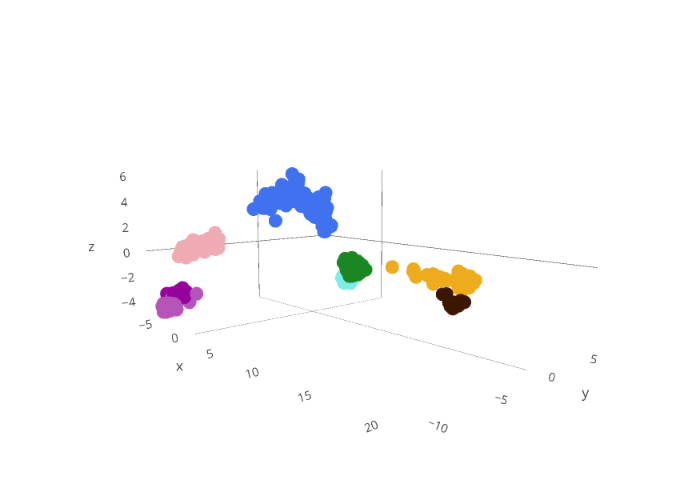
First let's look at the "genetic space" of the small cabbage white butterfly
Each point below is an individual butterfly.
The closer the points are together in this 3-dimensional space, the more similar they are genetically.
Each individual is assigned to a unique genetic group (represented by different colors) that was determined using an evolutionary model that tries to predict how many groups there should be and then assigns each individual to one of those groups.
If you scroll over them you can see each individual's ID# (if you participated in our project this will be your Pr_#), the country it was collected, its sex and the genetic cluster it was assigned to.
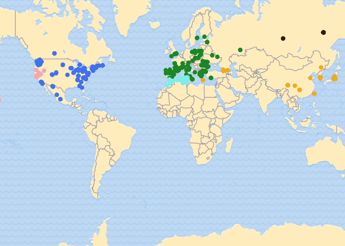
How are these genetic groups geographically distributed?
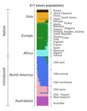
Here we aggregate individuals into their most likely genetic grouping (population). From our data it appears there are at least seven distinct populations. On the left, each horizontal bar represents an individual butterfly and is colored proportionate to the amount of the genome that was assigned to a particular population. Why do some individuals (bars) contain multiple colors? That individual's genome is likely a mix of different ancestries. That is, different parts of their genome come from different populations.
Step 3. Identify the historical routes of invasion
So why do we care about a species' invasion history? There are many reasons, from the practical--it can helps us manage their spread (e.g., helps us determine their natural predators) and possibly identify traits or conditions that allowed this species to rapidly expand its range.
How do we begin to figure out where an introduced species came from? We can start with observations. When and where they were first spotted? In the case the small cabbage white butterfly, we are fortunate that people, even in the 1860s, were paying attention to what species of butterflies were around them and often which ones seemed to be newly arrived. (click here to see how the entomologist Samuel Scudder used citizen science to reconstruct the spread of Pieris rapae across North America). With these observations we can make hypotheses about where a newly introduced species might have originated, using knowledge of the other places it is known to inhabit and the trade routes that might have helped to move the species to new locations.
Fortunately, the DNA in every butterfly retains some information that we can use to test some of these alternative hypotheses (scenarios). We can do this using a basic fact--the more DNA two individuals share in common, the more closely related they are. That means, if we have two different populations that we think might be the source for a new (introduced) population, we would expect that the actual source population will be the one that has more DNA in common with the introduced population. Think of it as a paternity test. The introduced population is the child and we are trying to find the parent from a pool of many possible parents (potential source populations). This is similar to how researchers and companies such as 23&Me use your DNA to learn about your ancestry. The difference being we are working with a butterfly =)
However, looking at genetic similarity alone can sometimes be misleading. That's because it doesn't account for how evolution can produce a diversity of patterns, depending on the conditions (scenario) that a population might have experienced. Luckily, advances in computing allow us to simulate the many different scenarios that could have led to the genetic patterns we see today. That is, we can create a simplified environment where we allow populations to evolve freely, guided by conditions specific to a scenario we have created. Think of it as "evolution in a bottle" with the bottle being an environment created by a computer. How do we know what scenarios to use? Ideally we would have some idea of what was possible and more importantly what was not possible. We can use historical observations--perhaps someone mentioned the species in a text or painted them into a picture and in so doing captured their location and time period, or maybe fossils have been discovered. Using this information we can create as many versions (scenarios) of history that we think might have been possible.
All scenarios begin from a point in time in the past where there was a single population. This population represents the common ancestor to all populations found today. Starting from there, we simulate the evolution (splitting) of this population into as many populations as are found today (this includes all potential source and introduced populations). For each scenario, we can simulate this process thousands or even millions of times. Each time, tweaking the conditions just slightly to add some "noise" (think of it as natural variability). We can then compare these simulated versions of what happened and see how well they match the genetic patterns we see today.
Dealing with uncertainty
It is often impossible to know for certain what happened in the past or what will happen in the future. Therefore, we usually want some measure of just how uncertain we are of the predictions made from the models we use to describe the natural world.
Take for instance climate change. When researchers use global climate models they include parameters they think are important. For example, climate models can include parameters for clouds, rainfall, evaporation, and sea ice, but also those dependent on human behavior such as trends in greenhouse gas emissions, reforestation, etc. Altering these parameters can alter a model’s predictions of future climate.
Similarly, for the model we used to infer how the cabbage white spread across the world we use a number of parameters that we know to be important, such as how large each population was prior to its introduction, whether it went through a bottleneck during its introduction and for how long, and when (i.e., the year) the introduction occurred. All of these parameters can influence how populations evolve and thus alter our expectation of what a population should look like (genetically) given a certain invasion scenario. Take for instance the date of first observation. This date is the date a species is documented for the first time somewhere outside its range. However, it is possible that the species has been there for quite some time already. Indeed, it seems quite likely that a half dozen small white butterflies might have gone unnoticed when they first arrived. Such is true for most invasive species.
One method for dealing with our uncertainty of the parameters we use in our models is to use a range of options (values) for each parameter. Usually we select a range of possible values based on what seems reasonable, an educated guess. For example, for the number of butterflies that were introduced we might choose values between 1 – 200 butterflies. We can then measure how the results change when the values of this parameter are varied. The range of estimates (predictions) output from our model reflect the range of possibilities for what might have happened. Essentially, the broader the range, the greater our uncertainty. However, because we simulate this outcome many times, we will inevitably predict the same outcome multiple times, thereby allowing us to look at which estimate was most common—e.g., the median estimate (this is what we have done).
Assessing the global invasion history of Pieris rapae
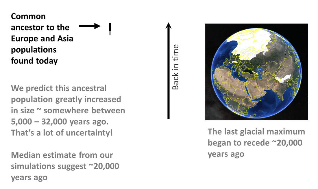
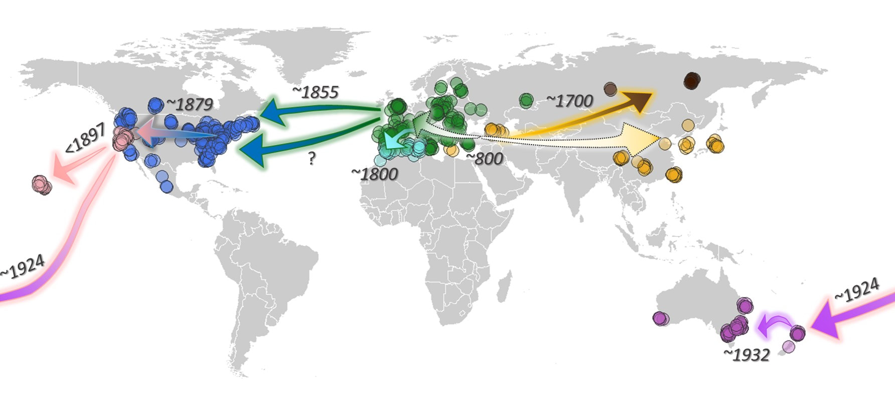
We applied this approach to uncover the global invasion history of the small cabbage white butterfly. First we knew that the oldest observations of Pieris rapae come from Europe and Asia. What we did not know was whether the population in Asia came from Europe, or whether the population in Europe came from Asia. That is, which population was the source for the other? The answer, as it turns out, is neither. But before we get into that, lets look at the ancestral population--the population that all contemporary populations can be traced back to (remember, you can think of it as the last common ancestor). One of the interesting things we found from our simulations was that this population underwent a dramatic increase in size about 5,000 - 32,000 years ago (that's a lot of uncertainty!). We don't know what caused this population to proliferate, but our median estimate for this event was 20,000 years ago and if true would coincide with the end of the last glacial maximum. Many species expanded their range as glaciers receded during this time period and it is possible that the small cabbage white did the same.
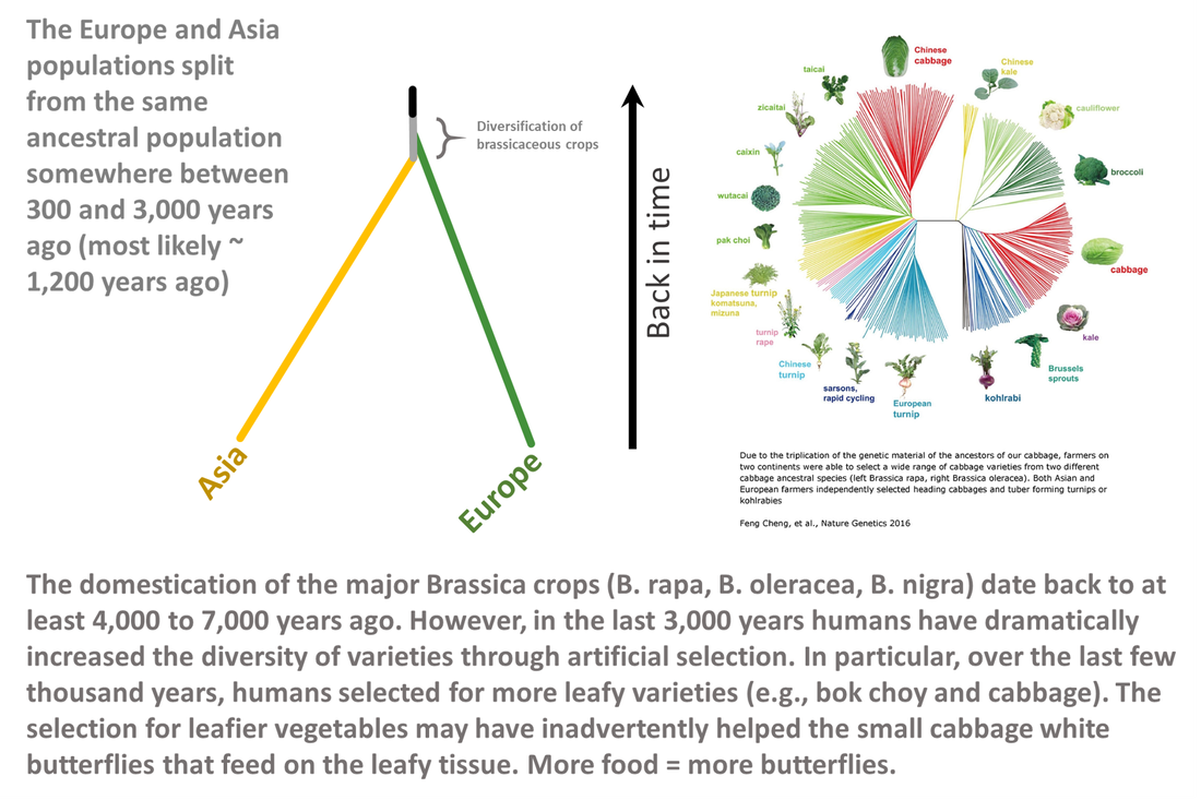
While many believed that Europe was the source for Asia we instead find that the most likely scenario was one where both Europe and Asia branched off from the same (ancestral) population. We predict this occurred about 1,200 years ago (800 CE). This time period overlaps with the increase in domestication of brassicas--the food of the caterpillars of small cabbage white butterflies. In particular, Brassica oleracea and Brassica rapa were experiencing an increase in cultivation. It is widely hypothesized that the diversification (selection for leafier varieties) of brassicaceous crops helped the small cabbage white to proliferate and spread across Eurasia and our results support this hypothesis.
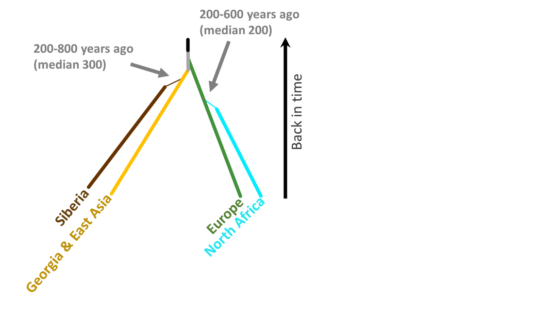
Our analysis also suggests that a very small population branched off from Asia and into eastern Russia about 300 years ago.
One hundred years later (200 years ago) a small population in Europe made its way to North Africa, possibly through Spain.
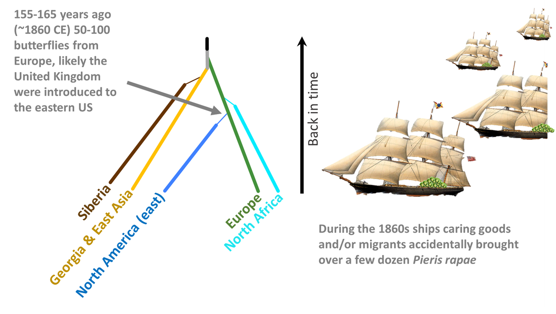
It is widely hypothesized that the small cabbage white butterfly was introduced to North America from Europe (United Kingdom), given the thousands of ships carrying goods and migrants were making their way from Europe to eastern North America during the 1860s. Our analyses suggest that this was in fact the case. It also appears that there was more than one ship carrying a few stowaways that arrived during the early stages of the invasion, just as Samuel Scudder's data suggest.
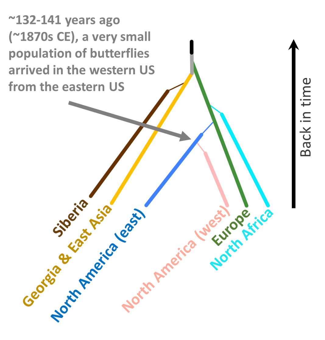
Interestingly, during our analysis we found a population in the western United States (centered in San Francisco, California) that is genetically distinct from other butterflies found in North America. We explored a number of different scenarios--this population came from Asia, from Europe, from eastern North America, or from Spaniards during the 1600s. Turns out, the most likely scenario is that this western population came from a few individuals that made their way west from eastern North America. Interestingly, when we looked at the development of railroad lines in North America during the time period that this population was predicted to arrive (~1879), we saw something interesting...take a look at see
Development of railroad lines in the United States from 1830-1972. Note the completion of railroad lines connecting eastern and western US in 1872, a few years prior to when a small population originating from North America (east) was believed to be introduced to North America (west) (i.e., central California).
|


